Contour Plots
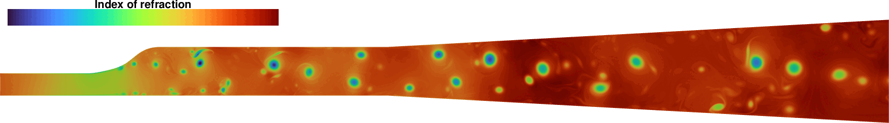
Now, let’s plot the dilute index of refraction using pyvista.
# Add the index of refraction to the mesh
internal_mesh.cell_data['n'] = index_of_refraction['dilute']

plotter = pv.Plotter(window_size=[1800, 900])
plotter.view_xy()
plotter.add_mesh(internal_mesh, scalars='n', cmap='turbo',
                 reset_camera='True', show_scalar_bar=False)
plotter.set_background('white')
plotter.camera.zoom(2.0)

plotter.add_scalar_bar(
    title='Dilute Index of refraction',
    title_font_size=22,
    label_font_size=18,
    bold=True,
    position_x=0.02,
    position_y=0.6,
    width=0.3,
    n_labels=8,
    height=0.1,
    vertical=False,
    fmt=""
)

plotter.show()
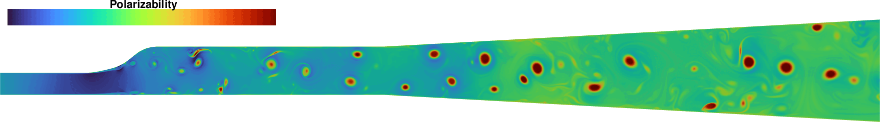
Now, let’s plot the Kerl polarizability using pyvista.
# Add polarizability to the mesh
internal_mesh.cell_data['pol'] = kerl_polarizability

plotter = pv.Plotter(window_size=[1800, 900])
plotter.view_xy()
plotter.add_mesh(internal_mesh, scalars='pol', cmap='turbo',
                 reset_camera='True', show_scalar_bar=False)
plotter.set_background('white')
plotter.camera.zoom(2.0)

plotter.add_scalar_bar(
    title='Polarizability',
    title_font_size=22,
    label_font_size=18,
    bold=True,
    position_x=0.02,
    position_y=0.6,
    width=0.3,
    n_labels=8,
    height=0.1,
    vertical=False,
    fmt=""
)

plotter.show()
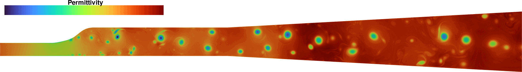
Now, let’s plot the permittivity of the medium using pyvista.
# Add Permittivity constant to the mesh
internal_mesh.cell_data['permittivity_dilute'] = permittivity_dilute

plotter = pv.Plotter(window_size=[1800, 900])
plotter.view_xy()
plotter.add_mesh(internal_mesh, scalars='permittivity_dilute', cmap='turbo',
                 reset_camera='True', show_scalar_bar=False)
plotter.set_background('white')
plotter.camera.zoom(2.0)

plotter.add_scalar_bar(
    title='Permittivity',
    title_font_size=22,
    label_font_size=18,
    bold=True,
    position_x=0.02,
    position_y=0.6,
    width=0.3,
    n_labels=8,
    height=0.1,
    vertical=False,
    fmt=""
)

plotter.show()
Now, let’s plot the electric susceptibility using pyvista.
# Add Electric Susceptibility constant to the mesh
internal_mesh.cell_data['susceptibility_dilute'] = susceptibility_dilute

plotter = pv.Plotter(window_size=[1800, 900])
plotter.view_xy()
plotter.add_mesh(internal_mesh, scalars='susceptibility_dilute', cmap='turbo',
                 reset_camera='True', show_scalar_bar=False)
plotter.set_background('white')
plotter.camera.zoom(2.0)

plotter.add_scalar_bar(
    title='Susceptibility',
    title_font_size=22,
    label_font_size=18,
    bold=True,
    position_x=0.02,
    position_y=0.6,
    width=0.3,
    n_labels=8,
    height=0.1,
    vertical=False,
    fmt=""
)

plotter.show()
